Point Cloud Processor Command

Command Licensing and Default Menu Location
- The Point Cloud Processor command is part of the RPS Tool Shed Toolbox
- The command is located on the Tool Shed macros menu ribbon
- The command is located in the QA / Point Clouds menu group
***
Command Description
Provides the ability to create a significantly reduced point cloud scan from an existing point cloud using smart gridding / binning and boundary techniques to reduce point density / quantity while retaining project surface model integrity and accuracy. Automatically builds surface model(s) from the resulting scan and boundary objects. You can now also use the Lowest Mode to eliminate vegetation and tree canopy from point clouds
Video Demonstration
The following video shows how to utilize the Process Point Cloud command
Latest Updates
March 6th 2023
The command was updated as follows
- Fully implemented the Lowest and Highest option - previously only the Mean option was activated. The Lowest and Highest option will store the true 3D location of the Lowest or Highest point in each grid cell. This means that when using Lowest, you now have an effective means of extracting ground and eliminating grasses, shrubs, bushes and tree canopy from point clouds. To eliminate vegetation, specify a smaller grid cell size for the max and min grid cell size than you would normally do e.g. 2’ and set the size so that it is likely to catch at least one ground point through the canopy of the vegetation. If you set the grid size too small, it is less likely to find a ground point. If you set the grid size too large you will smooth the surface more which may be less desirable. When you are removing vegetation, set the Elevation Range tolerance = 2x the height of the vegetation you wish to remove - in reality you can simply enter a large value here e.g. 1000 to eliminate all vegetation. You will still get a few spikes no doubt, but they will be easy to clean up using the Point Cloud menu tools.
Be selective about the areas that you wish to process for vegetation removal - while this is a great tool, if you want the most accurate terrain model on e.g. stockpiles or soil / dirt mounds. you will still be better off using the settings as before.
- We have also added a stronger control for the TBC Maximum points in surface setting, however it does appear that after we have adjusted the setting, TBC Options Manager is not updating when you open that control dialog - that appears to be a bug / defect on the TBC side that we have reported to Trimble.
September 21st 2022
We updated the command to add some additional error checking for the issue associated with the number of points from a point cloud used in a surface model (Support - Options - Point Clouds - Maximum number of points in surface definition). Currently until a user changes this setting, there is a default value that gets used, however it is not available in the Options list for a project / system installation. This trips up the Point Cloud processor command - hence the fix. In addition, we were finding that you could select a point cloud region or regions, however the Default Point Cloud region was non selectable, that also has been addressed.
September 7th 2022:
We added some additional support for the South Azimuth coordinate system. If you run the command in a project / project template from the command line and type RPSPCProcessor SA you will set a setting on that project that will from that point on offer you the ability to reduce the point cloud but also write a South Azimuth PTS file (where the E and N coordinates are multiplied by -1), so that on reimport of the file it will be located in the South Azimuth location for the point cloud. When the SA version is run, you will find this additional section in the command dialog.

The Adjust points for South Azimuth checkbox triggers the multiply the E and N coordinates by -1.
The Use South Azimuth adjusted points tells the command to import the South Azimuth adjusted data into the project rather than the North Azimuth unadjusted data. Both files are written as PTS files into the RPS folder of the project. The South Azimuth file has the suffix SA.
September 2nd 2022
We have updated the command to v5.70r12 to fix the reported issue that the reduced point cloud was shifted in relation to the original data. The issue was caused by the PTS Export / Import process when the project has a scale factor (Ground to Grid Scale Factor). The PTS export was using the Grid coordinates of the project, however the PTS importer assumes that the data is unscaled and adjusts it for the project scale factor thereby causing the shift in the data.
We now write the PTS file in two different ways depending on whether or not the project has a scale factor in play
- With a scale factor in play, we write the PTS file as a scaled up Ground Coordinate file to the users Temp folder with an extension other than .PTS so that it is clearly not a PTS file. We then import that file using the PTS importer that scales it back using the Project Scale Factor so that the data matches perfectly.
- Without a scale factor in play, we write the data as a PTS file into the RPS folder of the TBC project folder as Grid coordinates. Because the project Scale Factor is 1.0, the data is unadjusted during import so that the data matches perfectly.
Note that an imported PTS file is used in the determination of the project centroid (Elevation and Position) which is used to determine the project scale factor. The imported PTS file is in the same coordinate range as the original, but because of the decimation of the points, the distribution of the points could cause a minor change in the project centroid determination. That change could cause a minor change to the project scale factor, it is not likely to be significant.
Command Pre-Requisites
Before running the command, please go into Support - Options - Point Clouds and change the Maximum Number of Points in surface definition setting to any number other than the default setting i.e. the default is 500000 points, change it to 550000 or 1,000,000 etc. This will force TBC to write the setting into its Options file. If you do not do this the command may run but on execution, it may not do anything.
For large Point Clouds greater than 100 million points, you may want to run the Point Clouds - Sample Region command using Random mode down to 100 million points or less prior to running Point Cloud Processor on the results of that process.
In Support - Options - Project Management, check that you have the Use Project Subfolders checkbox enabled - if you have a project open and that is greyed out and unchecked then you do not have a Project Subfolder for the project and as a result there is no where for TBC to create the Point Cloud Database that is used to hold all point cloud data - when the Point Cloud processor runs it will create the Point Cloud Scan data but fail to import it as a result. To fix the issue, close all projects, go to Support - Options - Project management and enable the check box. Now any new project that you create will have this enabled and the Point Cloud Processor will work well. This setting is a good one to have turned on, we are not sure when / why you would ever not want a Project Subfolder, and cannot give you a good reason to ever turn this setting off.

Command Interface Description
The Point Cloud Processor command dialog looks as follows

Points / Point Clouds:
Select the point data or point cloud scans / point cloud region objects that you want to process
Maximum grid size:
The processor starts by dividing your selected data into “grids” which are squares of point data. Within each grid square the processor analyzes the variance of data from a height perspective. If the height variance in the square is greater than the elevation range tolerance specified, the grid is subdivided into 4 squares and the process is repeated. This process continues until all of the point data in the resulting “sub grids” are within the elevation range tolerance. It then takes an average elevation of the points in the resultant grids and creates a single point at the mean location of the data with that average elevation. Note that where a grid cell is at the edge of the model and the data is found towards one edge of the grid cell, the mean location will create the point in the center of the point data not in the center of the grid cell.
The result of the process is that on large flat areas where the elevation variance is minimal, you will have less data spaced at the maximum grid size, and where you have surface areas that are sloping you will have more data closer together so that the resulting scan data accurately represents the surface undulations or slopes.
Enter the Maximum Grid Size for the processor - we recommend using a grid size of e.g. 50’ or 25’ (20m or 10m) as a starting point to get a good distribution of points over large flat areas and to minimize the “rounding or smoothing effect” that could be created at the tops and toes of slopes.
The maximum grid size and the elevation range tolerance work in tandem to determine the degree of “smoothing” that the resultant surface will receive - i.e. a large grid size with a small elevation range tolerance (less smoothing) will create more points than a large grid size and a larger elevation tolerance (more smoothing).
Note that if you want to generate a fixed grid of result data, enter the same number into the Maximum Grid Size and Minimum Grid Size data fields. If you are using the command for vegetation stripping from the point cloud, enter a grid size that is relatively small but not so small that the processor is unlikely to find a ground point in each grid cell i.e. a grid size of 2’ will be better than a grid size of 1.0’. Note that a larger grid size will result in more rounding of the surface, a smaller grid size will result in a surface that more closely resembles the actual ground situation - so find the right balance. Remember that you can create different point cloud regions that you can process separately and with different settings and then merge the results together at the end to generate the best possible outcome. When vegetation stripping use the smaller grid size in combination with an Elevation range tolerance value that is greater than 2x the height of the tallest vegetation that you are trying to remove from the point cloud.
Here are some examples from a LAS file that initially contains 22,339,395 points to give you some examples

Here is an example section through two surfaces - exaggerated vertically that shows the original point cloud all points vs the thinned point cloud at 12.5’ grid and 0.25’ elevation tolerance

The following image shows the two surfaces in 3D - the Green surface is the original point cloud - all data points and the second grey surface is the thinned point cloud - reduced data points - you can see that the grey and green are continuously changing all over the surface giving a high degree of surface correlation within the elevation tolerance specified.
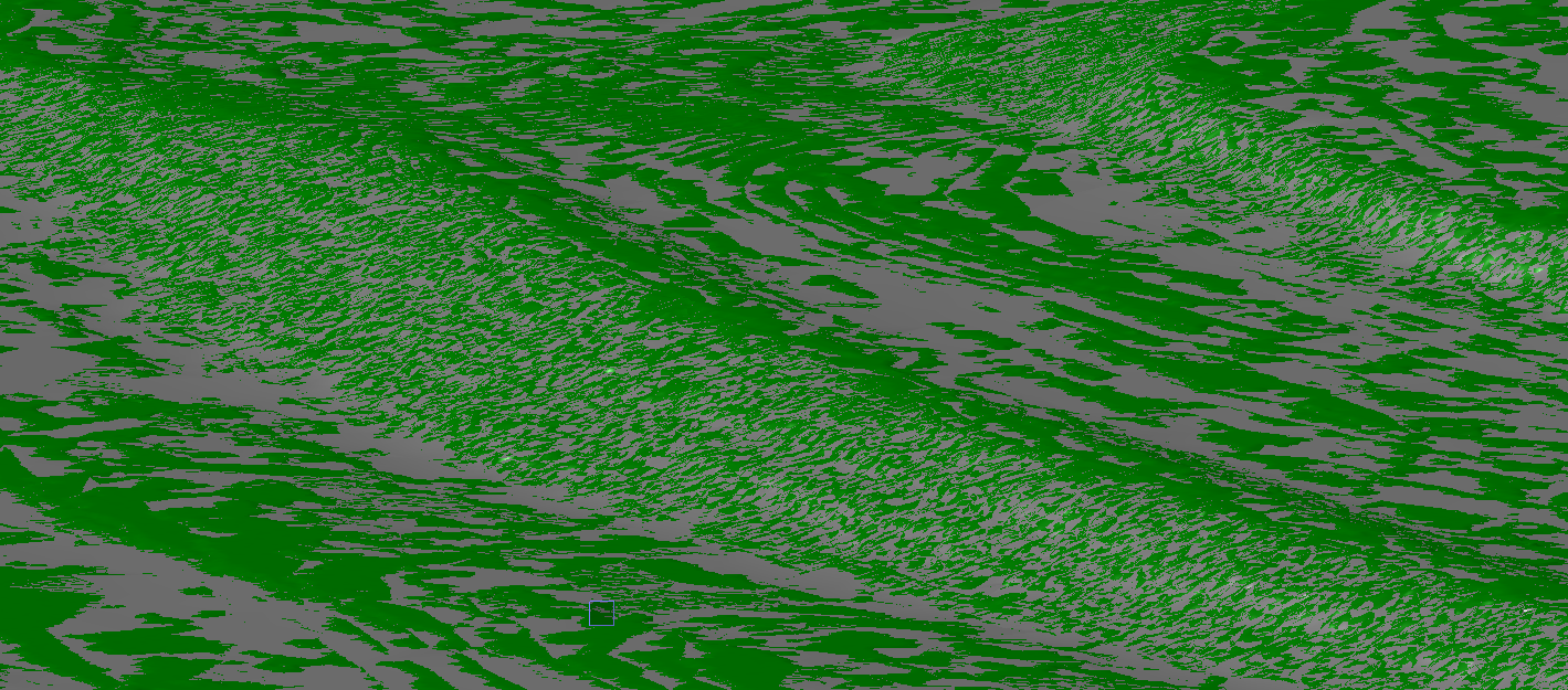
You can see from this data that the elevation range tolerance has the greatest impact on the point cloud data reduction, however the starting grid size will create more points over the larger flatter areas and will model around the tops and toes of embankment areas better / closer to original if it is smaller when the elevation tolerance is larger.
Whatever method you use to reduce the point cloud is a smoothing process, so the resultant surface will never be exactly the same as a surface created from all of the original source data points, the key is to ensure that for volume purposes, that the high and low smoothing balances approximately equally so that the cuts vs fills are all but zero balance. In the above images you can see that in the 3D view and the surface slicer views.
Minimum grid size:
The processor will continue to subdivide the maximum grid size until all of the point data in the grid falls within the elevation tolerance. If you wish to limit the grid size subdivision, you can enter a minimum grid size here, that will stop the calculations at that point and return the mean point elevation of the remaining points in the average position of the data in the cell (when using Mean Z coordinate mode). Note that edge cells where the data may not fill the entire area of the cell, the mean position is used, not the cell center for the created data points. If the subdivided grid cell fails the tolerance check it will be reported in the analysis pane at the end of processing. If you are using the Lowest or Highest Z coordinate mode, the actual location of the Lowest or Highest point is retained to avoid low / high biasing of the data that can adversely effect the result.
Elevation range tolerance:
The elevation range tolerance is used to determine the sub gridding of the data. The tolerance entered is a tolerance that is spread equally above / below a horizontal plane or a tilted plane if the “Fit planes where possible” checkbox is enabled. All of the points in a grid cell are analyzed against the plane to determine the variance of the points, if greater than the specified tolerance then the grid is subdivided and the process repeated. if the points analyzed lie within the tolerance then a point is determined at 4 quadrant points at 25% in from the edges of the grid cell and are then stored into the point cloud scan created.
When a horizontal plane is found to fit the point cloud data within a grid cell, a single point at the cell center is created with the average elevation of all the points in the grid cell (when using the Mean Z coordinate mode). When the horizontal plane fails to fit the data, a best fit plane through all of the points in the grid cell is determined, and all points validated against the tilted plane. If the tilted plane fails the grid cell is subdivided. If the grid cell passes the tilted plane analysis, 4 points are determined at locations 25% in from the grid cell edges. When using the Lowest or Highest Z coordinate mode, the actual 3D location of the Lowest or Highest point is retained and generated in the resulting point cloud.
Z coordinate mode:
In some cases, you may wish to create points in the grid that carry the highest or lowest elevation of the points analyzed. For example in Marine survey, they are most interested in the highest point of a scan because that is the point at which ships will bottom out on if within the depth range of the ships hull. The lowest Z coordinate mode allows you to find the Ground location in each cell and can be used to strip vegetation from the point cloud. Typically for earthworks we recommend using the mean elevation. For marine use the highest, and use the lowest mode for vegetation stripping purposes. When using the Lowest or Highest mode we recommend that you use a smaller grid setting and a large elevation range tolerance setting to get the best results. It also helps if the Max and Min grid size setting is set to the same value.
Fit planes where possible checkbox:
When checked, this changes the calculation from a horizontal plane to a horizontal and then tilted plane computation. When unchecked the calculations use a horizontal plane only for each grid cell for the sub gridding determination, this results in many more points being created on sloping surfaces e.g. on a 3:1 embankment. When checked, the same embankment points will be thinned more because the analysis now uses a tilted plane method to compute the thinning which will remove more points on sloped surface areas (where there is a consistent slope).
The tilted plane analysis is a secondary analysis on grid cells that fail the horizontal plane analysis. The tilted plane analysis is applied to a reduced data set created by the horizontal plane analysis.
When using the tool for vegetation stripping, there is typically no need to use the tilted plane calculation because you are working with a fixed grid size and trying to find the lowest point in each cell.
Cloud / surface name - Name prefix:
The process will create a point scan file and import it back into TBC as a new scan. The new scan will take the name of the source point cloud region used in the analysis and then add the entered prefix and suffix values to the name. e.g. if the original scan region was called Ground and you add a prefix AS-100-0.5- then the resultant scan name will be AS-100-0.5-Ground.
Cloud / surface name - Name suffix:
The process will create a point scan file and import it back into TBC as a new scan. The new scan will take the name of the source point cloud region used in the analysis and then add the entered prefix and suffix values to the name. e.g. if the original scan region was called Ground and you add a suffix “-Reduced” then the resultant scan name will be Ground-Reduced.
You can add a prefix and a suffix at the same time if required.
Inclusion boundaries layer checkbox and selection:
When you fly a site with a drone, the drone will inevitably cover areas outside the project limits. In addition the drone will fly over areas within the project that contain data that is non representative of the ground surface e.g. Material storage areas, laydown yards, a group of trees, wetland areas, buildings, parking areas for vehicles etc. It is likely that these areas will exist in each flight data set that you process. The Inclusion / exclusion boundary options allow you to draw inclusive boundaries and exclusive boundaries on separate layers in TBC and then use those here to further reduce the point cloud during processing.
Draw your inclusion boundaries on a layer and select the layer here by checking the checkbox and selecting the layer from the layer list pull down. Note that you can have 1 or more inclusion areas - these will become islands of point cloud data if you want to create islands of data e.g. the approach and departure embankments for a bridge under construction. The most typical use for an inclusion area is the site limits to exclude data outside of the boundary and include data within the boundary.
You cannot place an inclusion boundary inside another inclusion boundary without having an exclusion boundary between them.
Exclusion boundaries layer checkbox and selection:
Draw your exclusion boundaries on a layer and select the layer here by checking the checkbox and selecting the layer from the layer list pull down. Note that you can have 1 or more exclusion areas - these will become holes in the point cloud data e.g. in areas of tree groups or around parking areas or around material piles that exist in the current scan or in all data sets that you create from regular flight missions.
You cannot have an exclusion boundary inside another exclusion boundary without having an inclusion boundary between them.
Create surface(s) checkbox:
Once the point cloud scan has been created and imported, the point cloud can then be modeled into a surface or surfaces directly if required. Check this checkbox to create the surface or surfaces from the resultant point cloud scan.
Add inclusion boundaries to surface checkbox:
The inclusion / exclusion boundaries that you use to reduce the point cloud data can also be used to build the surface models. If you add the inclusion boundaries they will be added to the resultant surface as inclusion boundaries of the surface also.
Note that if you have two or more inclusion boundaries that separate two or more areas of a project with gaps in between, if you do not add the inclusion boundaries to the surface, the triangulation will form between the two areas of the point cloud.
Create separate surfaces for each inclusion boundary checkbox:
If you have more than one inclusion area you can use them to create separate surfaces e.g. if you fly a stockyard and create a point cloud for all of the stockpiles, you can create surfaces for each stockpile separately if you put inclusion boundaries around them.
Note also that if you have a large project area and you want to divide the survey into different phase areas that you can model with smaller numbers of points, you can use inclusion boundaries and multiple surfaces to achieve that.
Check this checkbox to create a separate surface from each inclusion boundary selected to create the thinned point cloud.
Add exclusion boundaries to surfaces:
If you cut out areas from the point cloud in the middle of the surveyed area, you can decide whether or not you want to use those same boundaries to exclude the surface in those areas.
If you are OK with forming the TIN model across the voided point cloud areas, do not check this check box and the surface will form between the points around the outside of the voided area across the voided area.
If you want to also void the surface in these areas, check the checkbox to void the areas in the surface model also.
TBC Maximum points in surface:
In TBC when you add a point cloud region to a surface it uses a setting found under Support - Options - Point Clouds called “Maximum points in surface” to extract a number of points randomly from the selected point clouds to form the surface. This setting is exposed here in the dialog so that you can change it for this process only (it does not permanently change the TBC setting, just overrides it for this processing execution). In this case you are first reducing the point cloud using the point cloud processor to create a reduced point cloud, that you likely want to use all of the points in the resulting scan to form a surface. The setting here can be set to a number above the estimated number of points that will be created using the settings provided to utilize all of the points created.
The results pane will show you messages like that shown below based on the settings provided and the point cloud selected. In the example shown, we have selected 3,000,000 points for the surface model - this is a large surface so we advise you that that may take time to create. In addition the estimated points in the resulting scan is between 4.4 million and 2.2 million so 3 million may be too low in certain situations so we warn you of that possibility. Note that the estimates are on the heavily conservative side - we typically see reductions of 90 to 98% whereas it is showing you 80 to 90% reduction ranges here).

Command Tips
The command tips provide you some information on dealing with Large Point Cloud data sets as follows " For large point cloud data sets, use the Sample Region command to reduce the point cloud to 100 million points or less (64GM RAM) or 50 million points or less (32GB RAM) before running the point cloud processor. " Also included is a reminder that F1 is your shortcut to this help document.
Header Commands
In the header bar of the command you will find command icons that link you to other commands that you may need access to while using this command. In this command the following commands are linked
- Help - this document access
- RPS Settings
- Takeoff Lines
- Smart Edit
- Adjust Linestring Elevation
- Create Boundary
- Point Cloud by Boundary
- Sample Point Cloud Region
- Create Point Cloud Region
- Add to Point Cloud Region
- Create Quick Contours
- Create Contours
- Label Contours by Crossing
Apply
When you tap Apply, the source point cloud is processed, a new reduced point cloud scan is created and imported. The command will ready itself for another selection set and repeat process execution. If you do not want to make a second selection and repeat the process tap Close to finish the process.
If the project has a scale factor (Ground to Grid) then the PTS file is written with a non PTS file extension to the users Temp folder before being imported. The PTS file is in Ground scaled coordinates.
If the project has no scale factor (1.0 Ground to Grid) then the PTS file is written with a PTS extension to the RPS folder in the current project’s project folder in the Grid coordinates of the original data.
Close
Closes the command without further execution.
Use Case Videos
The following videos show the use of the Process Point Cloud command in a work process context
This video shows how to remove Tree Canopy and brush from a Point Cloud using the Point Cloud Processor command. Note in this type of workflow you need to use a vertical tolerance greater than the height of the canopy or brush you are trying to remove i.e. for 3’ brush you need a tolerance of e.g. 8’ and for 60’ trees you will need a tolerance of e.g. 70’. There is no real harm in using a tolerance of 1000. In addition you want to select a Max and Min Grid size at which most grid cells analyzed will have at least a single ground point - selecting a very small grid size will minimize that likelihood, opening up the grid to 2 or 3’ will increase the likelihood depending on the density of the canopy.
In the next video we have looked at Lidar data and how we can use the Point Cloud Processor to effectively smooth the Lidar to create a “good” surface model. I think the results are pretty stunning - here is a surface made from all the points in a small sample area

Here is the smoothed data

Note the surface slicer view of the comparison - the grey line is the Mean Smoothed Surface and the Green Line is all the original data points surface. The noise level on the Lidar is ~ +/- 0.25’
Video provides more details
Feedback and Enhancement Requests
If you would like to provide feedback on the use of the Process Point Cloud command or to request enhancements or improvements to the command please click Reply below.